The idea
Recent skill improvements in meteorological and ocean forecast have been by incorporating observations into model predictions. Numerical model development, by means of improved physical representations, is in many cases suffering from diminishing returns. While ensemble approaches (many) models are useful and provide uncertainty estimates, the assimilation of ever increasing data into models is needed. The folks over at Google’s Deep Mind more recently showed that deep neural networks could be used to accurately predict short-term (up to 90-minutes) precipitation events using prior radar observations (Nature article). These predictions were more accurate than the high-end, complex, numerical weather models operated by the National Weather Service. While weather models still reign supreme for longer-term forecast, accurate short-term predictions are useful by forecasters during weather extremes.
Inspired in part by their success, and in part by my previous work with ocean wave forecasts (SWRL Net), I wanted explore the idea of making short-term corrections to operational weather forecasts of both wind and waves. Because winds create waves, wave observations may therefore be useful to wind forecasts and vice-versa. So in short: Can we make better short-term forecasts by learning corrections based on recent forecasts and observations?
The data
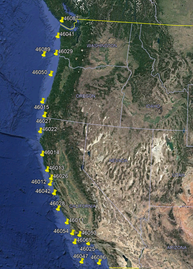
Floating buoys along the coast measure winds and waves. While these buoys exist all over the globe, I’ll start with just observations on the U. S. West Coast. The buoys, owned and operated by the National Data Buoy Center, NDBC, are located below marked by the yellow pins. While the deployment lengths vary, each buoy has several years or more of data for which to use.
A long-term model hindcast of winds and waves has been archived by the National Ocean and Atmospheric Administration (NOAA) that can be used as a proxy for operational forecasts (WW3 CFSR). Wrangling data from both NDBC and NOAA we will then have both a set of observed winds and waves, as well as forecasts.
First step
To keep things simple, we will first try to improve predictions of one component of the wind field (wind is a vector), in this case the $u$ component which is the speed in the eastward direction. The formulation of the model is relatively simple, such that
$$ u_t = M (u^o_{t-1}, u^f_{t-1}, u^o_a) $$
where we aim to make an improved prediction, $u_t$, at time $t$ with a model, $M$, that is a function of the observed wind, $u^o$, and forecasted wind $u^f$ at the prior time step, $t-1$. Additionally we will include the daily average observed wind, $u_a$. Now it would be a little limiting to examine just the prior time-step, and so instead we can include many prior time steps, up to $T$ such that
$$ u_t = M (u^o_{t-1},\ldots,u^o_{t-T}, u^f_{t-1},\ldots,u^f_{t-T}, u^o_a) $$
Similarly, predicting just one time-step into the future may be too easy, and we can include several, up to future forecast time-step, $F$, such that
$$ [u_t,\ldots,u_{t+F}] = M (u^o_{t-1},\ldots,u^o_{t-T}, u^f_{t-1},\ldots,u^f_{t-T}, u^o_a) $$
It is worth noting one, we will use hourly time steps as that is forecasted time step in NOAA’s hindcast, and two, that we really should work in a residual space, $u^r = u^f - u^o$, and instead develop a model for $u^r$. Nonetheless we will keep things simple for the moment, working with $u_t$ and revise the model later. Now the question becomes, what model should we use, and how well does it do?
In this first pass we can look at the simplest model, the linear regression, as well a multi-layer perceptron (MLP) network with 25-layers (additional layers lead to over-fitting). Splitting the data into a train and test set (for now we will skip the dev set) we can answer the first question, how well do these models preform? Root-mean-squared errors are estimated on the test set for each buoy (y-axis) and each hour forecasted into the future (x-axis) as shown below.
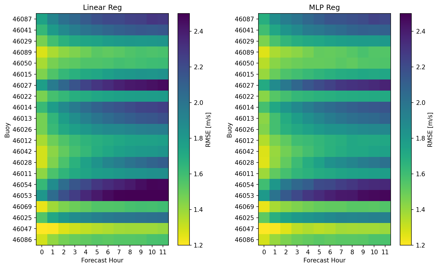
The left hand panel shows results for the linear regression while the right shows results for the MLP Network regression. Models have similar skills with some buoys have overall higher errors and others lower. There is a consistent trend that errors in the first few forecast hours are comparably lower. While that makes inuitive sense, there is yet, not context for these errors. The meaningful question is really, how do these errors compare to the original forecast? Surely they are not worse, are they?
It seems the model was correctly implemented and we observed only improvement in RMSE. Shown below is the percentage change in RMSE between the model prediction and the original forecast.
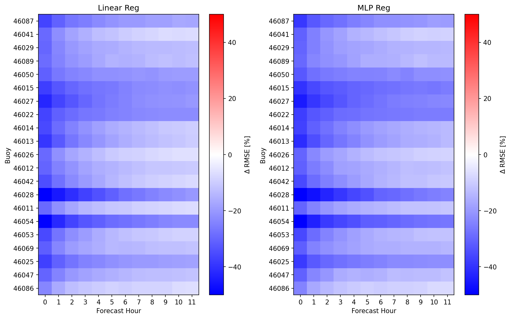
Here, for most buoys we observe a 20-50% reduction in error for the first few forecast hours with a 0-20% reduction present in later hours. It becomes more apparent that the MLP Network is producing slightly better corrections to the forecast that tend to persist for longer. While the differences are not huge, it is good to see that the 5-hours spent training those models have yielded something positive (note the linear regressions fit in a trivial amount of time)
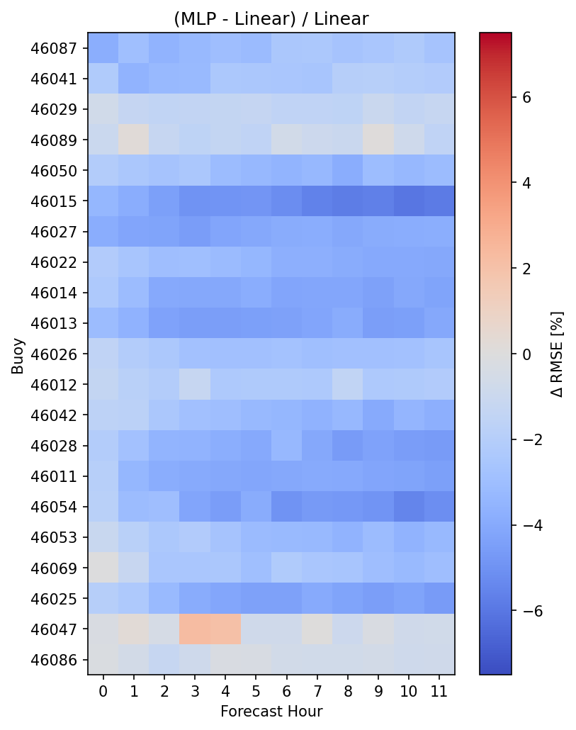
Exactly how much improvement was observed? Well we can estimate that, again as a percentage. The MLP network appears to reduce RMSE by about 2-6 percent compared to the linear regression, with only a couple buoys and forecast hours showing worse errors. However, there is clearly room for improvement.
Woah, let’s back up a little
So far we see that we can make some skill improvements over typical model forecasts by training on prior observations and future forecasts with a linear regression, and finding some added skill moving to a neural network, but let’s come back to the linear problem and ask a few simpler questions, such as do we need all the inputs we are providing? Should we include the historical forecast as well? What does each part of the feature puzzle bring us in terms of skill as a function of forecast hour?
To take a look at these questions I’ve created several linear models with varying inputs, ranging from just the yearly average, to including both the historical forecast, historical observations, and future forecast. Now the plots below shows all these combinations with the right plot just a zoom in on the y-axis to see the differences between the best models a little more clearly.
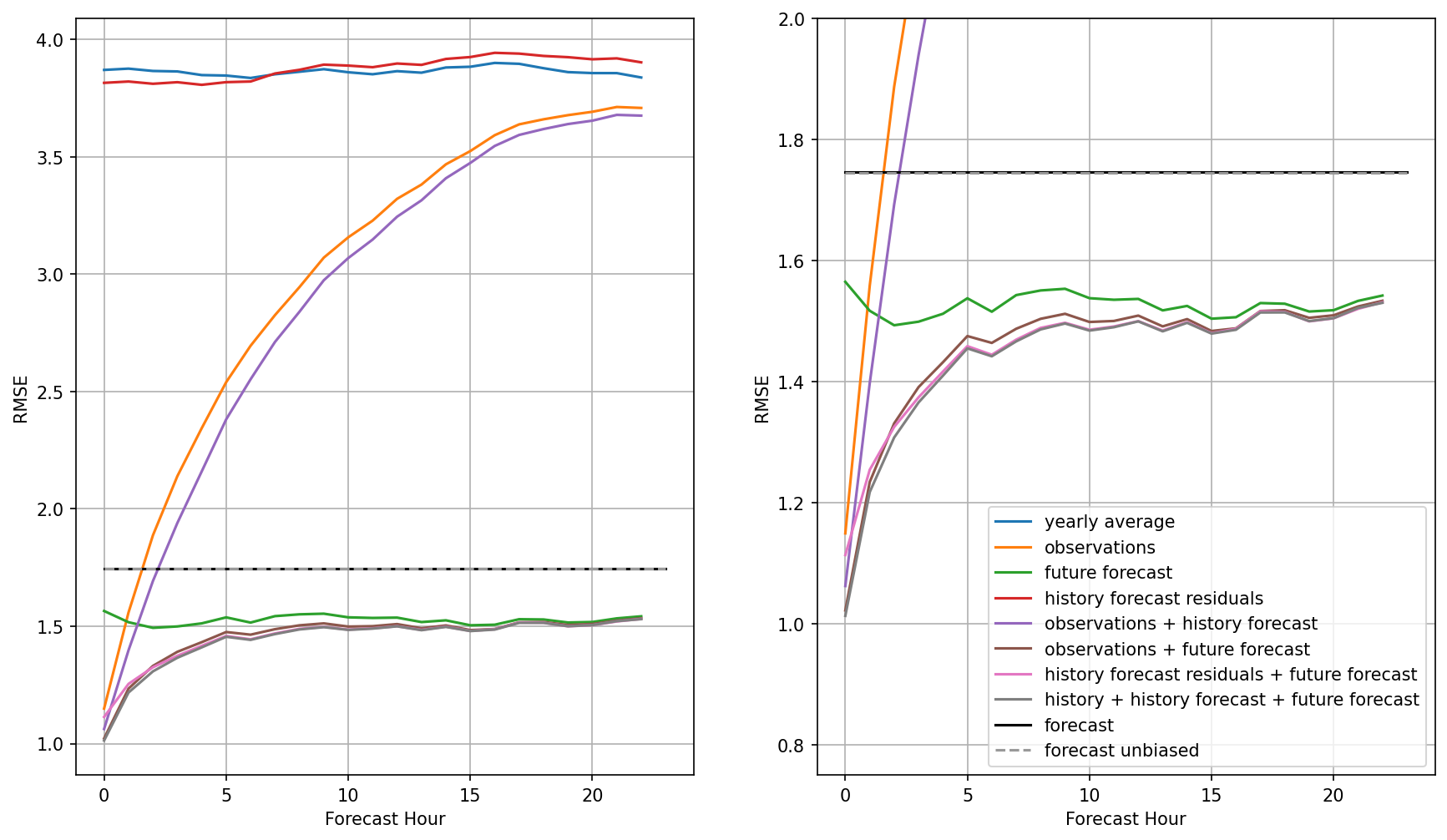
Let’s start with the worst models. First training with just the yearly average estimate does a poor job, to no surprise with an error of about 3.9 m/s. This is a far cry from the original forecast error around 1.72 m/s (black line). Now similarly bad is the model trained on the history forecast residuals. By residuals I mean the errors in the forecast in the last 24-hours, e.g. forecast - observations. This at first seems surprising, but the model has little context for which to learn from just the past errors with no reference to the current wind speed magnitude at all. You really can’t do much with the error term alone. Now the next thing to try is just the observations (orange). Here, we have good skill at forecast hour 1 and 2, with skill much worse in the preceding hours. Again, this is intuitive as the model probably is guessing that wind conditions are similar to the latest hour, which works for a short time.
Now, what about just providing the model future forecasts? In this case we see a relatively constant RMSE around 1.5 m/s. This is not surprising as we created mock forecast from hindcast that therefore have similar skill for all forecast hours, however, what is surprising is that this skill is higher than the forest itself, and higher than the bias-removed forecast. Clearly some averaging is happening here that is helpful.
Now, we start to see how our more general linear model starts to put together the pieces. By including both prior observations and future forecasts we get a combination of improvement at early hours and at later forecast hours. Various combinations of observations, history forecast residuals, and future forecast hours result in similar curves, with best results given the larger number of parameters. We are not necessarily over-fitting, however, because these results are derived from the test set.
Since we have a linear model we can explore it’s coefficients relatively easily. What of these inputs are actually useful? First let’s just consider the relatively simpler linear regression with historical observations and future forecasts. Taking a look at the coefficients (here negatives are historical observations, positives the forecast hours) we see a relatively inutitive set of coefficients for various forecast predictions.
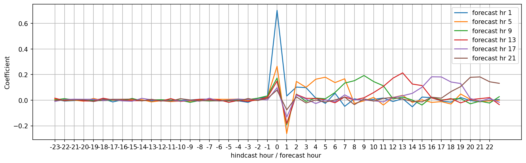
Here for forecast hour 1 the coeficient of hour 0, the latest observation, is 0.65, or in other words, the regression would like 65% of this hour followed by a little bit of the most recent forecasts. For later forecasts we see less reliance on the latest observation and more reliance on the forecast hours nearby those forecast hours themselves. Now a linear regression with an L1 penalty and a little regularization shows us which coefficients are actually useful.
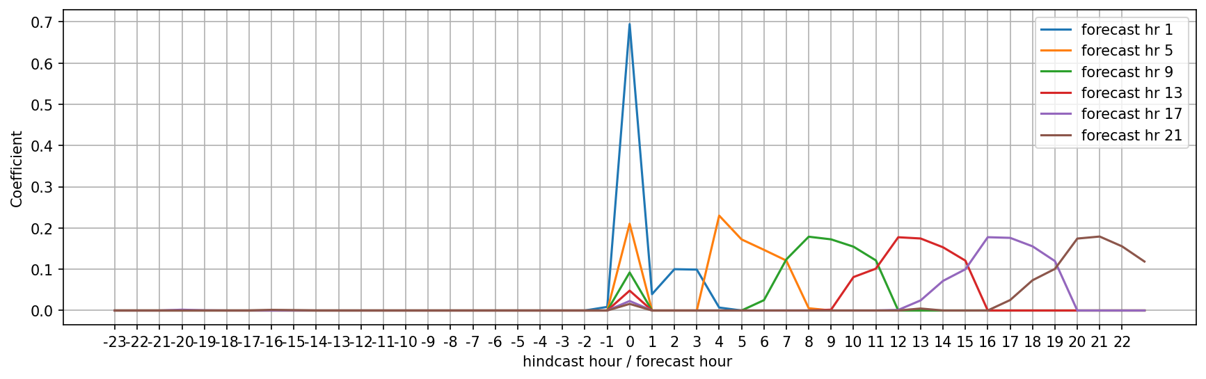
Here, we see that indeed the model cares only for the latest observation, the first forecast hour, and then an average of the forecast hours surrounding the desired prediction forecast. The shape of this averaging is relatively consistent and interestingly asymmetric. This is actually the preferred averaging window that should, in theory, improve the forecasts! Interesting, and I wonder how it might vary from observation location to observation location. What is also quite surprising is that earlier observations are not useful.
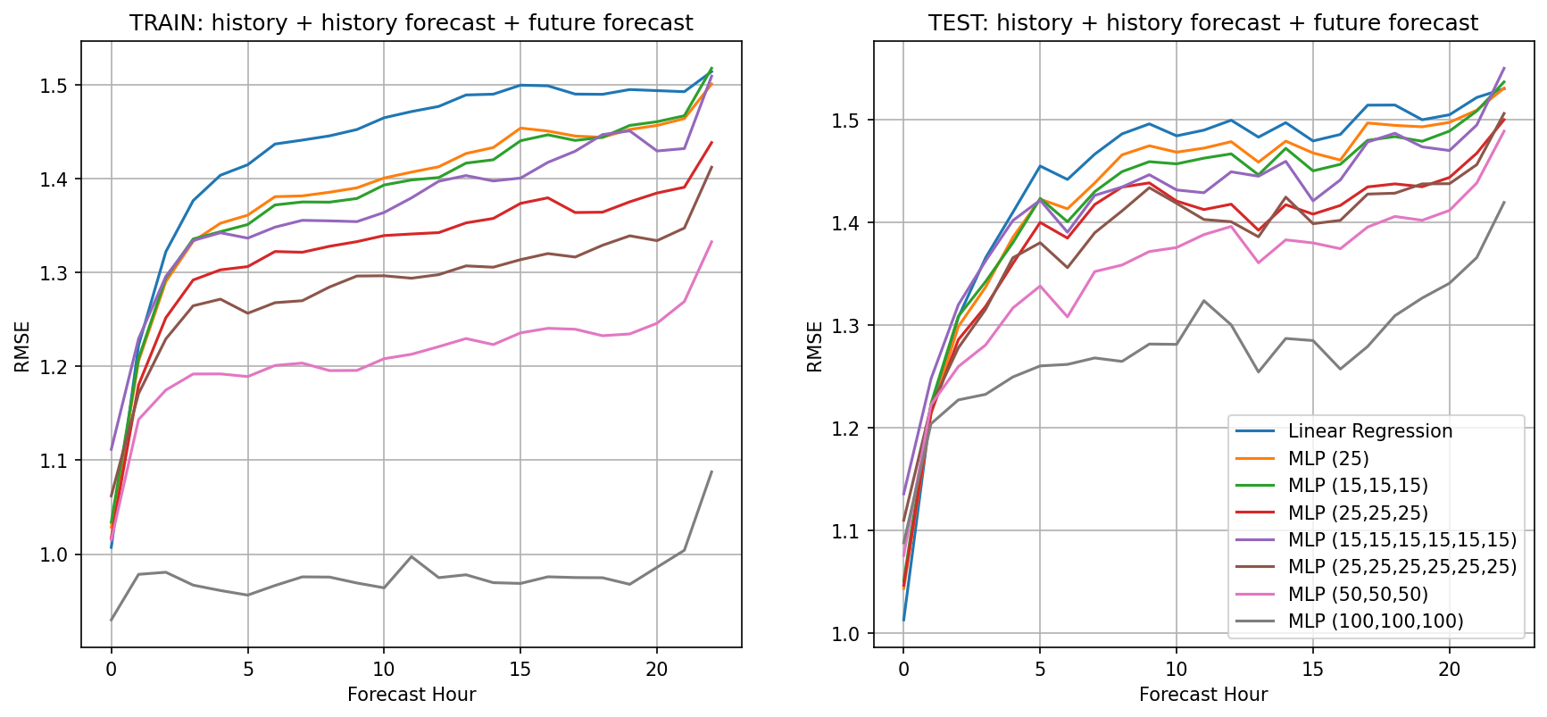
Now that we explored the linear regression in a bit more detail let’s go back to the multi-layer-perceptron model (aka neural net) and start with the inputs from our best linear model, that is observations + historical forecast + future forecast. I think we can conclude that the average daily wind speed was not useful. Using default settings that include RELU activation, adam for the solver, a small amount of regularization (.0001) let’s try varying the amount of layers and their nodes. While training becomes a bit slow (about 5-minutes for the largest network) we can see clearly that deeper networks with an increasing number of nodes appear to reduce RMSE, increasing prediction skill. And this improvement is relatively constant across forecast hour, which is a pleasant surprise suggesting that possibly we should consider predicting farther than 24-hours out. What is also clear is that the models are indeed over-fitting as training errors are much lower than test errors.
Next steps
This cursory examination suggests there is potential to reduce forecast errors and several avenues for further exploration including
- Examine linear coefficients for a model with history forecast as well (or residuals)
- Explore regularization and/or other approaches to reducing over-fitting with MLP
- Split into train-dev-test, and consider splitting by dates to avoid potential overlap
- Modeling $u$ and $v$ wind components together
- Adding wave forecast and observations to model inputs
- Scaling inputs if adding wave and observations
- Determine if MLPRegressor is automatically scaling, as it should be expecting 0-1 as inputs right?
- Consider grid search or other random search for optimal hyper-parameters.
- Exploring additional model architectures such as recurrent neural-nets
If you have ideas, send me an email!