Support Vector Machines (SVM) are seemingly derived from a intuitive concept, drawing a decision boundary with the widest margin (aka gutter, street, etc.). While this only really applies to the linear problem in which the data are indeed separable, I find it particularly helpful in visualizing the decision space of the model. Unlike a random forest or multi-layer neural network, it is easy to picture model space. While not a novel idea in the slightest, this provoked me to consider decision space for several classification algorithms to hopefully gain insight into other techniques, and with this insight select appropriate methods for future questions.
The toy dataset
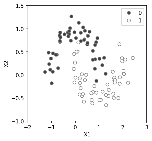
To visualize model space and the decision boundary of each classifier we will use a dataset with just two features. To make thing interesting let’s use a somewhat on-trivial dataset, the toy dataset generated with scikit-learn moons. The data form two half moons of 1 and 0 across two dimensions, call them X1 and X2 as seen here. Clearly a simple linear approach will not work well, but let’s see what happens as we start with the simple and move to the complex.
The logistic classifier
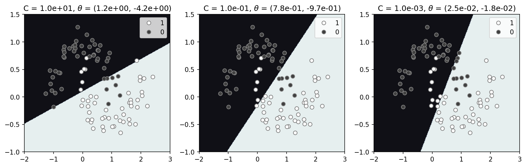
The simplest, I think, approach is a linear or logistic regression. For classification purposes we use the logistic regression to determine the probability of a given class. The decision boundary will be drawn at 0.5, separating the two classes 0 and 1. We have a regularization parameter, C, that we can employ to penalize large model parameter values ($\theta$). The model decision space below makes intutitive sense, separating both classes with a plausible straight line (left panel). Increasing the regularization (decreasing C) changes the orientation of this line and results in a slightly worse fit, missing more the data than with a relatively low regularization (C=1). In this case significant regularization does not appear to be needed.
Linear support vector classification (SVC)
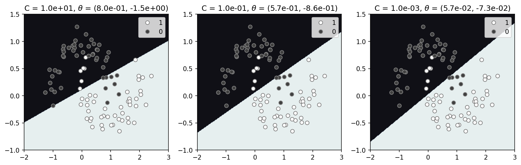
The linear support vector is employed here on data that is not linearly separable. So while the goal is the same, making a decision boundary with the largest street/margin/gap between the data, here we must allow for violations. Again, we have a regularization parameter C that has a similar impact as in the logistic classifier. With minimal regularization (left panel). Increasing the regularization, as in the logistic classifier, we see a similar affect on the decision boundary, but to a less severe degree. With little regularization (C=1) the solution appears nearly identical to the logistic decision boundary (left panels). I think we would expect stronger differences in a data if it was separable as the goal in SVC (widest street) differences from the logistic regression (minimizing least squares). I illustrate this in a notebook focused on the classic iris flowers dataset, notebook.
Non-linear support vector classification
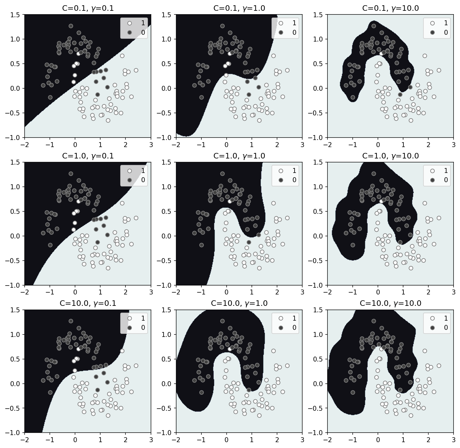
What’s really nice about SVMs is that we can relatively easily, and quickly utilize non-linear solutions (through the “kernel trick”) and still be guaranteed a convex solution space without local minimums. Here, the inverse of C still controls the regularization while an additional parameter $\gamma$, controls the degree of non-linearity. Increasing $\gamma$ allows for more wiggles to better fit the data, but this can of course, also lead to over-fitting. In the results above C=1.0 and $\gamma=1.0$ appear to be most reasonable solution to the solution space, which, likely by coincidence, are near default values. With significant regularization and minimal non-linearity the solution appears to converge to the linear SVC and logistic boundaries (top left panel). I should note that here we used the radial basis function (rbf), which is just one option for the kernel, and in this case the most reasonable, but it worth exploring the others.
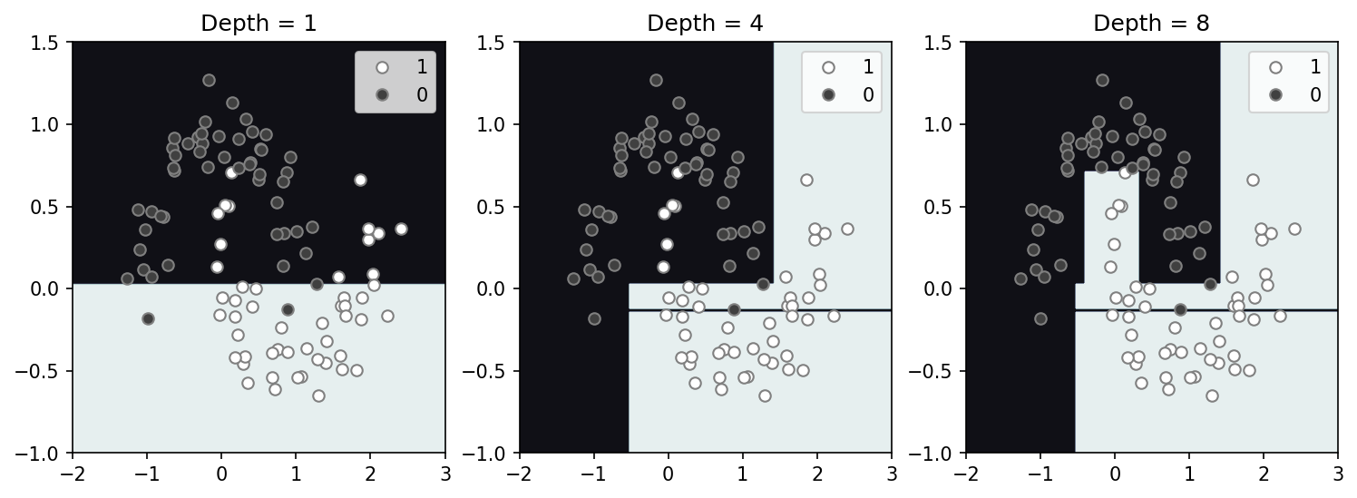
Decision tree
The decision tree is another relatively simple approach to classification that is a cascading set of decisions. These appear to manifest in an increasing complex gridded structure with a greater number of boundaries with increase depth. The solution below appears boxy, with a higher depth value allowing for additional boxes to be delineated. Increasing the depth tends to fit the data better but naturally can lead to over-fitting. Interestingly here, even with a low depth of 4, the model prefers to make a very narrow slice of 0-space to correctly identify a single 0 data point in a sea of 1’s. By eye this looks like an issue for generalization. Overall the gridded structure differs widely from the approaches previously discussed.
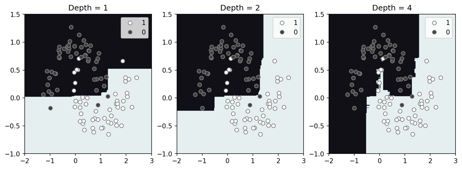
Random forest
A random forest is simply a large collection for decision tress that are created using random segments of training dataset. Decision boundaries are determined by which classification receives the most votes from all the trees. While this information can be additionally used to derive confidence in the solution, I’ll focus just on the decision boundary here. Here, using 100 trees trained on the entire dataset (no train/dev/test here) we create a model space shown below for varying tree depth. Interestingly, even with a shallow depth, we can map much more complexity than with the single decision tree. Some downsides that pop out immediately are that, (1) the results are random and will vary with iteration, and (2) over-fitting appears much more likely as there is significant fine structure with a depth of 4.
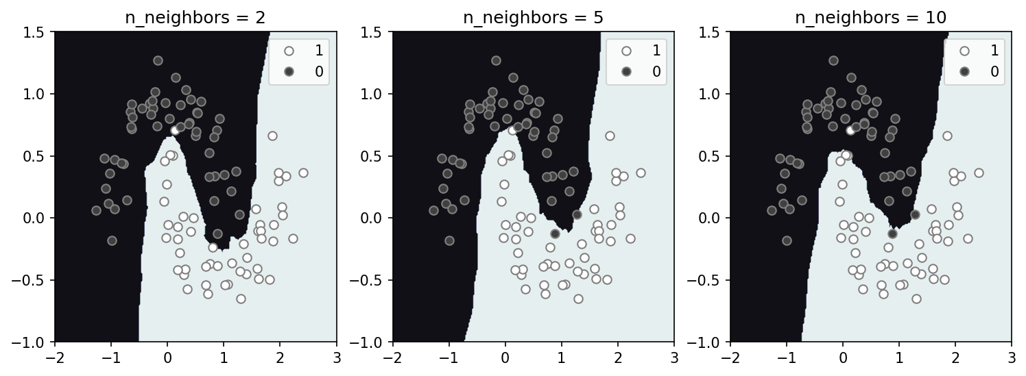
K-nearest neighbors
A comparatively simpler approach, k-nearest neighbors (Knn), simply maps decision space by querying the K-nearest data points and using the majority to determine the classification. Using a larger $K$ leads to a smoother, potentially more general solution that incorporates a larger amount of the data. A smaller $K$ leads to a better fit, but can risk over-fitting. Determination of a reasonable $K$ for a given dataset is critical, and varies. Below we generate solutions for a range of $K=2$ to $K=10$ (n_neighbors). Without additional data and a train-dev-test set it is difficult to determine an optimal $K$, however it is clear how a larger $K$ leads to solution space with slightly less features.
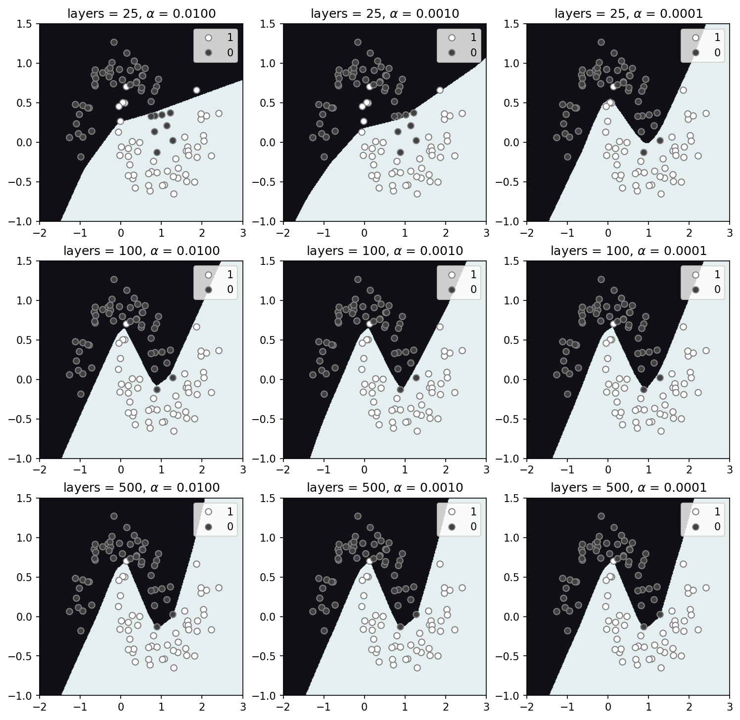
Multi-layer-perceptron (MLP) network
The neural network, here, has the largest number of trained parameters by far, and likely the most difficult to interpret. However, from the solutions below it is clear that a simple neural network prefers to make straight lines where it can. Here, the number of network layers vary with rows and the regularization parameter, $\alpha$, with columns. For 25-layers (top row) regularization has a strong impact, reducing the complexity and fitting far fewer data. For a larger number of layers model solutions are all relatively similar. Not being an expert of any kind, I cannot really comment on the results here, but I find it very interesting that solution space appears somewhat like a set of linear models, delineating the space with a small set of straight boundaries.
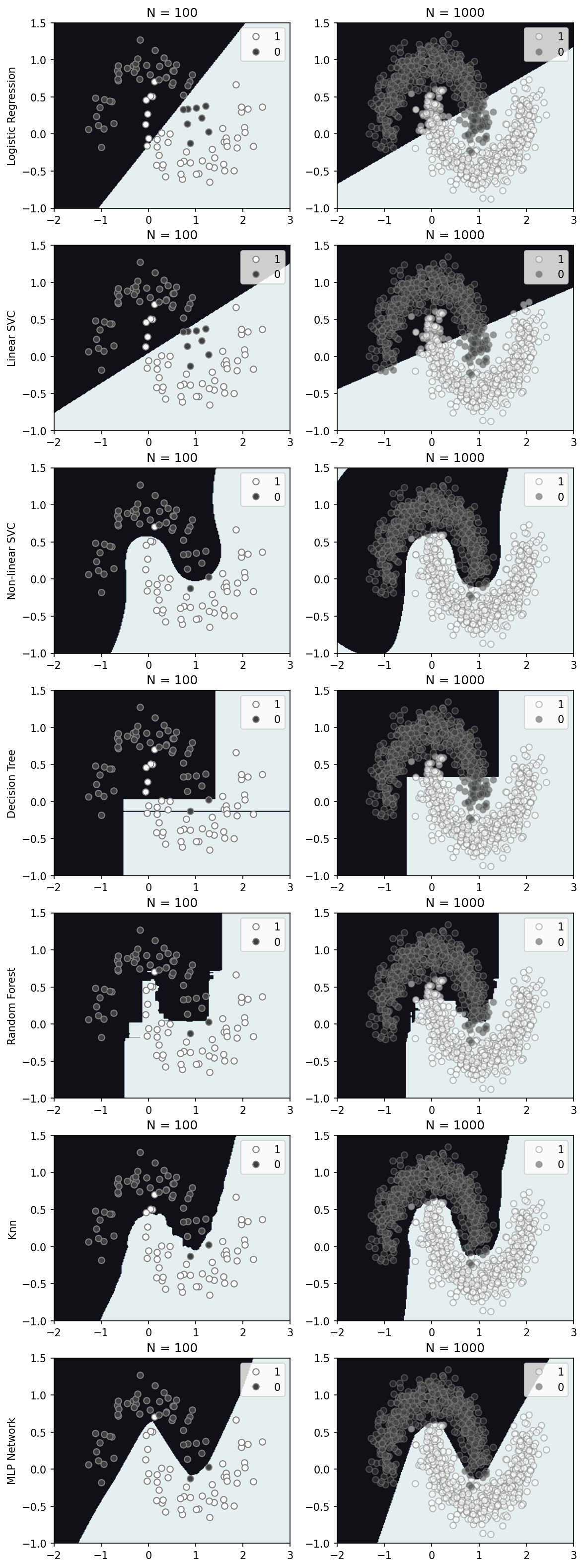
Adding data
Varying models and some of their parameters was interesting, but we can also vary the dataset size. In general, adding data tends to improve the decision space of the model. Interestingly, in this case, the models that vary the least with additional data are the linear and non-linear SVC and MLP network. I’d probably argue that the non-linear SVC may look the best, but with a train-dev-test approach I would not want to say what model is truly best. Clearly the solutions between models are different and do not tend to converge to a uniform solution with additional data (at least in the low data density regions), and that is what I find most interesting.
Summary
As this is simply a toy model, I wouldn’t take anything here very seriously, however, I find the decision space illustrated helps give me some intuition for how these model work and vary. Because this is a such a simple model (two features) it is difficult to say too much about how these generalize. For further reference and code, my python notebook can be found here, jupyter notebook.