Today I was wondering if I can make some sense of a rather large 60-year hindcast of winds in Washington around the Salish Sea. Could I see what the typical wind patterns in the region are? How can I manage this with a rather hefty 1+GB set of spatial wind predictions? This is a good opportunity to explore empirical orthogonal functions (EOFs), also known as principle component analysis (PCA).
Empirical Orthogonal Functions
What is an EOF? An EOF is the decomposition of a data set in terms of orthogonal basis functions. This set of basis functions will contain all the information in the dataset, but broken into empirical functions that are most different from each other (orthogonal) and account for the most amount of variance as possible. These are typically ordered by the amount of variance accounted for, with the most the first in the matrix. In my example here I have 1271 grid locations (a 31 x 41 grid) and 89,000 time steps.
Because of memory limitations, I’ve restricted the EOF analysis to 20,000 time steps. Generating the orthogonal functions is just a single line, calling a function to perform a singular value decomposition (svd, available in numpy.linalg). I provide my 1271 x 20,000 element matrix of wind predictions, call it W, and what I end up with is three matrices, U, S, and V, such that
$$W = USV^T ,$$
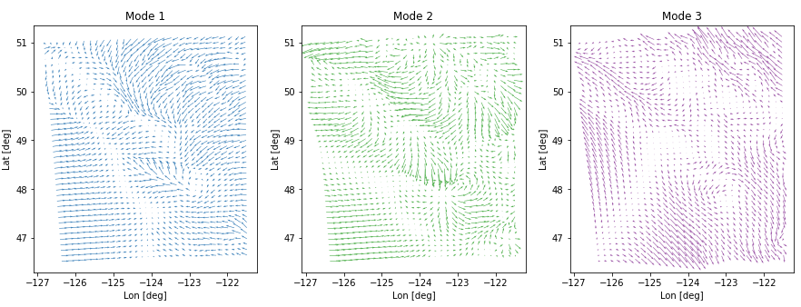
where U is 1271 x 1271 and is my set of orthogonal functions across space and V is similarly those functions in time (20,000x20,000). S is a diagonal matrix who’s values correspond to the variance represented by each orthogonal function. The variance of the first functions represent about 7, 7, and 5% (19%) of the overall variance. This might not be considered a lot, but nearly 20% of the spatial variability can be described by just 3 patterns! In this case 3 of the 1271 possible.
The geographical setting
Here you can see some relatively large patterns that are typical of the region. Mode 1 representing onshore flow from the ocean and offshore flow from land. Mode 2 shows similar onshore flow but with more southerly flow inland. Mode 3 shows a strong north flow offshore at higher latitudes and southward flow at lower latitudes showing a divergence region just below the Strait of Juan de Fuca. To help illustrate, for lack of basemap, the three modes are show below
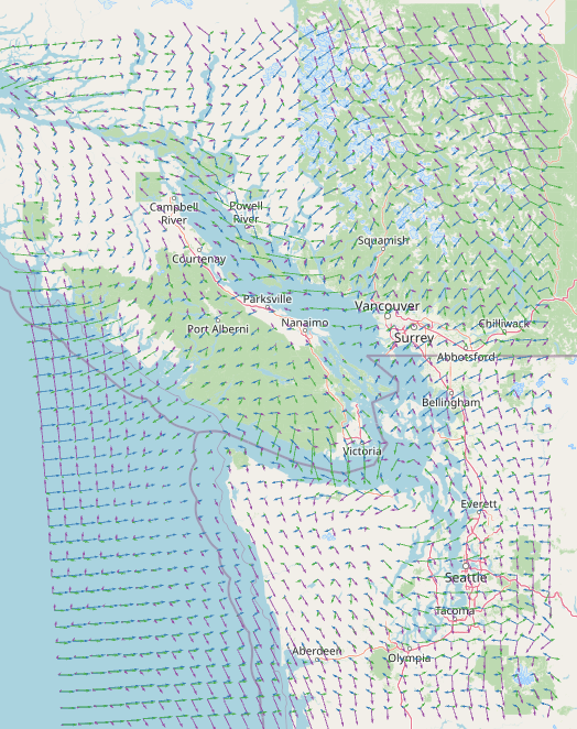
What I really enjoyed seeing was the effects of the Olympic mountains on winds just to the East. You can see what looks like a swirl in all of the modes. Wrapping up I’ll link an interactive html file here and the jupyter notebook used in the analysis described is here. If you’d like data please get in touch.
What makes it complex?
An aside that I didn’t mention above. Wind vectors have two components whereas what is described above assumes just a single value, like say winds speed. However, with a vector you can use complex notation to represent the two dimensions under a single matrix such that
$$\hat{u} = u + iv.$$
Here, the northward component, v, is imaginary. The computation is the same, but at the end you’ll need to take the real and imaginary parts to recreate the vector. And note that instead of normal transpose above, the hermitian transpose is need that additionally takes the complex conjugate of V.